xrspatial.multispectral.arvi

xrspatial.multispectral.arvi(nir_agg: xarray.core.dataarray.DataArray, red_agg: xarray.core.dataarray.DataArray, blue_agg: xarray.core.dataarray.DataArray, name='arvi')

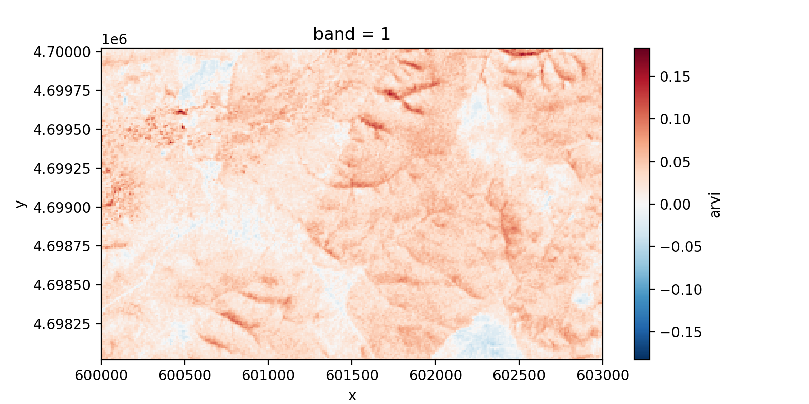
Computes Atmospherically Resistant Vegetation Index. Allows for molecular and ozone correction with no further need for aerosol correction, except for dust conditions.

Parameters

• nir_agg (xarray.DataArray) – 2D array of near-infrared band data.

• red_agg (xarray.DataArray) – 2D array of red band data.

• blue_agg (xarray.DataArray) – 2D array of blue band data.

• name (str, default='arvi') – Name of output DataArray.

Returns

arvi_agg – 2D array arvi values. All other input attributes are preserved.

Return type

xarray.DataArray of the same type as inputs.

References

• MODIS: https://modis.gsfc.nasa.gov/sci_team/pubs/abstract_new.php?id=03667 # noqa

Examples

In this example, we’ll use data available in xrspatial.datasets

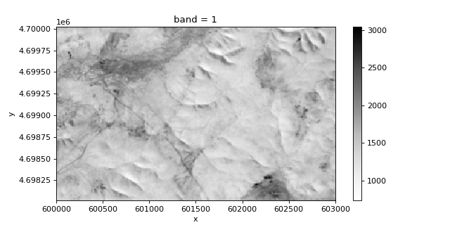
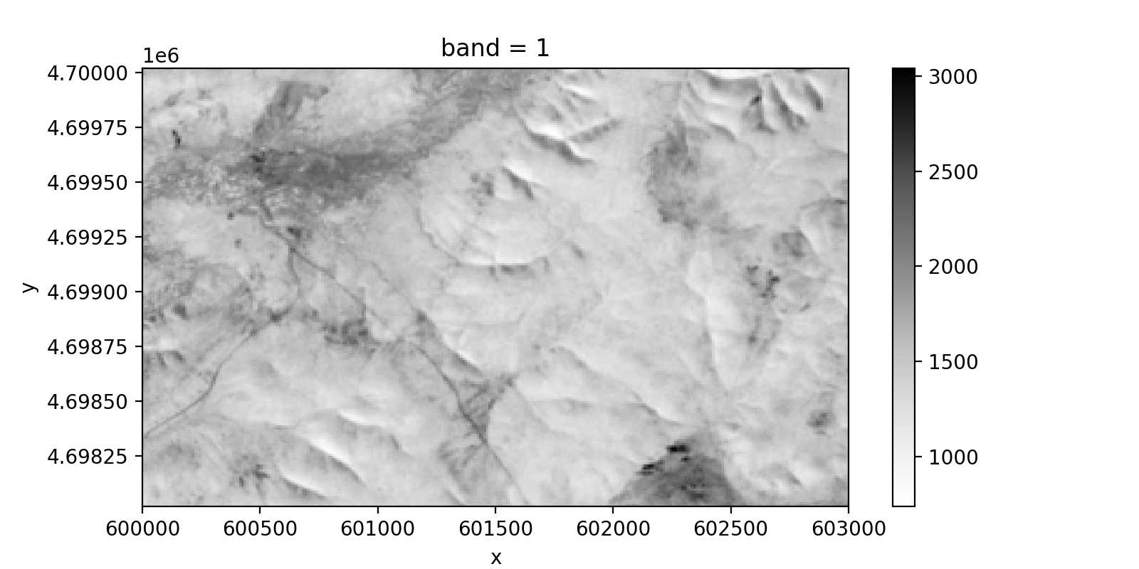
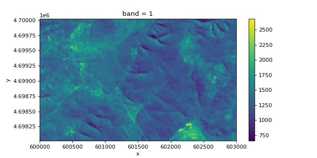
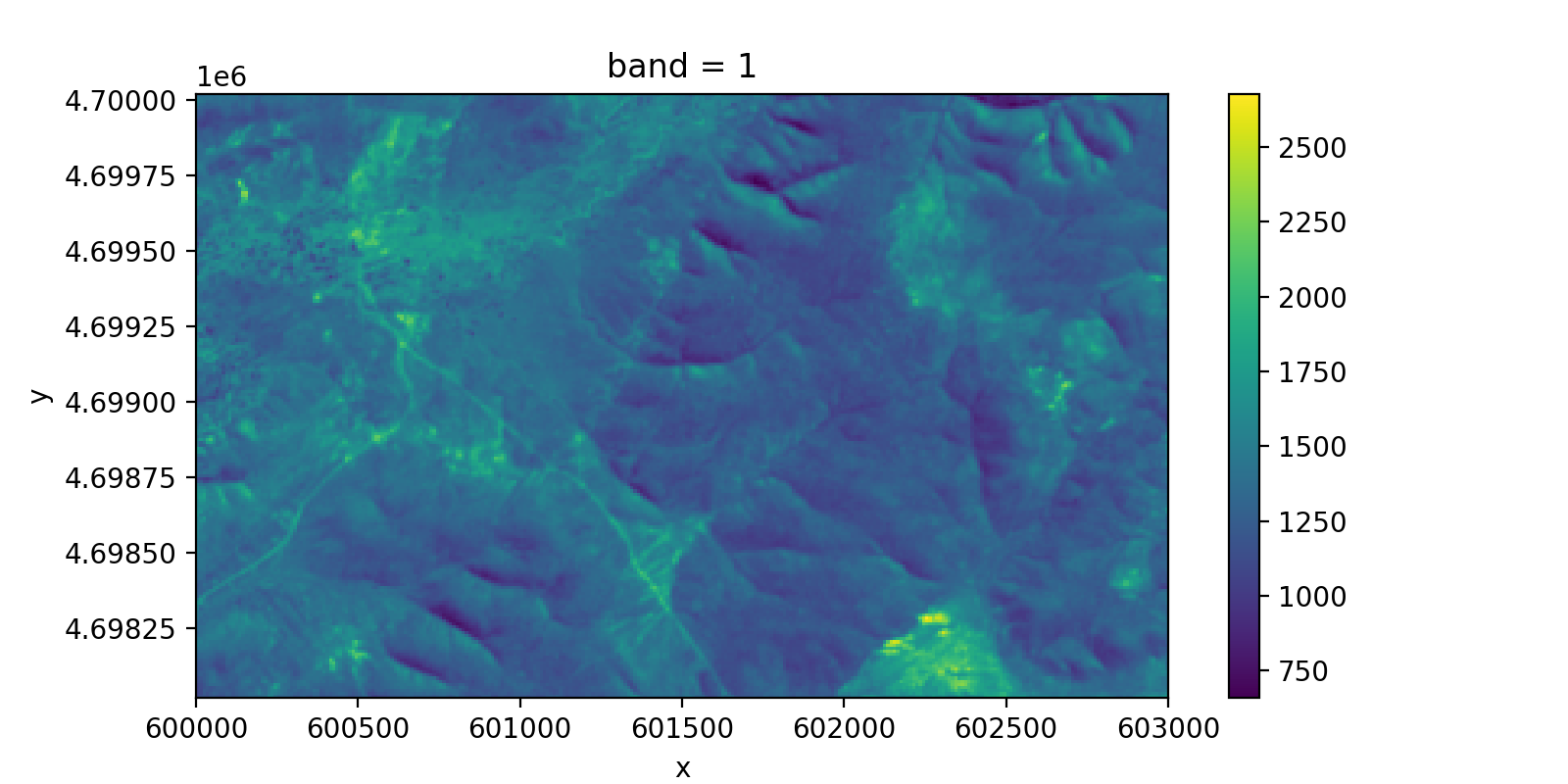
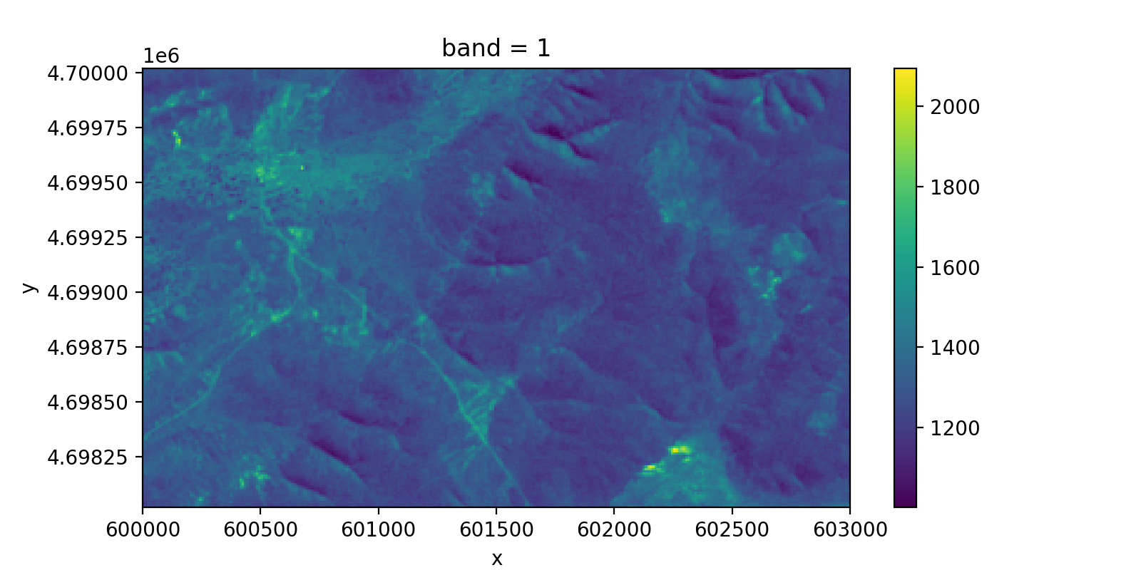
>>> from xrspatial.datasets import get_data
>>> data = get_data('sentinel-2')  # Open Example Data
>>> nir = data['NIR']
>>> red = data['Red']
>>> blue = data['Blue']
>>> from xrspatial.multispectral import arvi
>>> # Generate ARVI Aggregate Array
>>> arvi_agg = arvi(nir_agg=nir, red_agg=red, blue_agg=blue)
>>> nir.plot(cmap='Greys', aspect=2, size=4)
>>> red.plot(aspect=2, size=4)
>>> blue.plot(aspect=2, size=4)
>>> arvi_agg.plot(aspect=2, size=4)

(png, hires.png, pdf)

(png, hires.png, pdf)

(png, hires.png, pdf)

(png, hires.png, pdf)

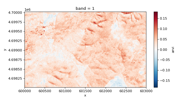
>>> y1, x1, y2, x2 = 100, 100, 103, 104
>>> print(nir[y1:y2, x1:x2].data)
[[1519. 1504. 1530. 1589.]
 [1491. 1473. 1542. 1609.]
 [1479. 1461. 1592. 1653.]]
>>> print(red[y1:y2, x1:x2].data)
[[1327. 1329. 1363. 1392.]
 [1309. 1331. 1423. 1424.]
 [1293. 1337. 1455. 1414.]]
>>> print(blue[y1:y2, x1:x2].data)
[[1281. 1270. 1254. 1297.]
 [1241. 1249. 1280. 1309.]
 [1239. 1257. 1322. 1329.]]
>>> print(arvi_agg[y1:y2, x1:x2].data)
[[ 0.02676934  0.02135493  0.01052632  0.01798942]
 [ 0.02130841  0.01114413 -0.0042343   0.01214013]
 [ 0.02488688  0.00816024  0.00068681  0.02650602]]